快速入门
快速入门部分简要介绍了Scorecard-Bundle的重点功能:特征离散化、WOE编码、离散化调整、特征选择、评分卡模型训练/调整、模型评估、模型结果解释。用户可据此快速开发评分卡模型,但实践中往往需要一些小技巧以应对的多种困难(例如特征数量较多时对全量特征进行离散化计算成本高、离散化调整人工成本高等)。评分卡建模的最佳实践请参考完整代码示例。
- 与Scikit-Learn相似,Scorecard-Bundle有两种class,transformer和predictor,分别遵守fit-transform和fit-predict习惯;
- 使用Scorecard-Bundle建模的完整示例展示Example Notebooks
- 详细用法参见API Reference;
- 注意Scorecard-Bundle中的特征区间均为左开右闭区间。
模块导入
from scorecardbundle.feature_discretization import ChiMerge as cm
from scorecardbundle.feature_discretization import FeatureIntervalAdjustment as fia
from scorecardbundle.feature_encoding import WOE as woe
from scorecardbundle.feature_selection import FeatureSelection as fs
from scorecardbundle.model_training import LogisticRegressionScoreCard as lrsc
from scorecardbundle.model_evaluation import ModelEvaluation as me
from scorecardbundle.model_interpretation import ScorecardExplainer as mise
特征离散化(ChiMerge)
Scorecard-Bundle在特征离散化步骤采用ChiMerge算法(由Randy Kerber发表于"ChiMerge: Discretization of Numeric Attributes")。ChiMerge属于bottom-up的离散化算法,基于特征的分布和目标变量在特征不同取值的相对频率对相似的取值进行合并,最终得到统计上有显著差异的区间。离散化步骤将数值型特征离散化为序数型的区间、或将序数型特征的相似取值合并。分类型特征需先转化为序数型才能进行离散化(例如可以通过响应率排序为分类型特征编码)。
Scorecard-Bundle的ChiMerge模块默认采用等频分箱作为前置步骤,以避免直接应用ChiMerge输出的特征区间容易在样本规模上高度不平衡的问题(部分区间只有少量样本)。
如下所示,可首先实例化一个ChiMerge实例,并用数据训练得到最终离散化区间。max_intervals 和min_intervals 参数控制输出区间的数量、decimal 参数控制区间阈值的小数位数。其他参数的介绍请见API Reference
trans_cm = cm.ChiMerge(max_intervals=10, min_intervals=2, decimal=3, output_dataframe=True)
result_cm = trans_cm.fit_transform(X, y)
trans_cm.boundaries_ # see the interval boundaries for each feature
与sklearn中的任意transformer一样,ChiMerge支持:
fit(): 训练。得到最终离散化区间。e.g.trans_cm.fit(X,y)transform(): 基于学习到的离散化区间阈值,将特征原始值转化为离散化区间。e.g.trans_cm.transform(X)fit_transform(): 训练并将原始值转化为离散化区间。e.g.trans_cm.fit_transform(X,y)
若需要按用户自定义的离散化区间转化特征,可使用assign_interval_str()函数,详细用法和示例见"离散化调整"步骤。
特征编码(WOE)
证据权重 (Weight of Evidence, WOE) 是目标变量的局部分布和全局分布的商的自然对数,反映了全局事件率与每个分组的局部事件率的差异,这意味着编码的数值与特征值对目标变量的区分能力呈线性关系,因此对特征进行WOE编码可以使回归模型更好的捕捉非线性的关联关系。
信息值 (Information value, IV) 在WOE编码的基础上进一步计算得到,是用于评估特征的区分能力的常用指标。IV值可在WOE_Encoder训练后可由属性iv_获取。
其他参数的介绍请见API Reference。
trans_woe = woe.WOE_Encoder(output_dataframe=True)
result_woe = trans_woe.fit_transform(result_cm, y)
print(trans_woe.iv_) # information value (iv) for each feature
print(trans_woe.result_dict_) # woe dictionary and iv value for each feature

# IV result
res_iv = pd.DataFrame.from_dict(trans_woe.iv_, orient='index').sort_values(0,ascending=False).reset_index()
res_iv.columns = ['feature','IV']
离散化调整
评分卡模型通常期望入模特征具备如下特点:
- 特征须具备基本的区分能力(e.g. IV>0.02);
- 特征的分布不应过于不均衡(e.g. 特征值不应对应过少的样本);
- 特征的响应率曲线通常为单调或二次方(U型),以便于人类理解模型表现出的关联关系;
- 响应率曲线的趋势与特征取值分布的趋势应不一致。从统计角度上看,假设一个特征对于一个目标变量没有区分能力,样本规模较小的特征值比样本规模大的特征值更可能对应更低的响应率,这种现象在目标变量分布不均衡时尤为明显。因此当响应率曲线的取值与特征取值分布的趋势一致时,我们常常不能确定样本规模小的特征值具备较低响应率是因为该特征确实对目标变量有区分能力,还是响应率低仅仅是因为特征值覆盖的取值范围较小、不易匹配到数量较少的目标变量为正的样本;
在离散化调整步骤,应查看单个特征的取值分布和响应率分布,调整取值分组使特征能更好的满足上述期望。
查看分布和响应率
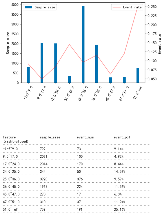
使用plot_event_dist() 函数可以方便的将特征分布可视化,包括每个特征值的样本分布和响应率分布。
  col = 'housing_median_age'
  fia.plot_event_dist(result_cm[col],y,x_rotation=60)
修改特征分组
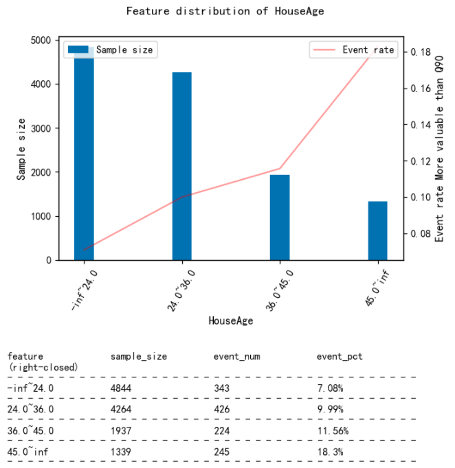
基于上面的特征分布分析可确定新的特征分组阈值,使特征的分布更加理想。使用 assign_interval_str()函数可将用户自定义的阈值应用于特征原始值,得到离散化的特征分组。
new_x = cm.assign_interval_str(X[col].values,[24,36,45]) # apply new interval boundaries to the feature
woe.woe_vector(new_x, y.values) # check the information value of the resulted feature that applied the new intervals
({'-inf~24.0': -0.37674091199664517,
'24.0~36.0': -0.0006838162136153891,
'36.0~45.0': 0.16322806760041855,
'45.0~inf': 0.7012457415969229},
 0.12215245735367213)
再次查看分布图
fia.plot_event_dist(new_x,y
                  ,title=f'Feature distribution of {col}'
                  ,x_label=col
                  ,y_label='More valuable than Q90'
                  ,x_rotation=60
                 ,save=False # Set to True if want to save to local position
                 ,file_name=col # filename in the case saving to local position
                 ,table_vpos=-0.6 # The smaller the value is, the further down the table's pisition will be
                   )
更新分组特征数据
将调整后的特征更新至离散特征数据集中。完成全部入模特征的离散化检查和调整后,此数据集将经WOE编码后用于逻辑回归的训练。
result_cm[col] = new_x # Update with adjusted features
feature_list.append(col) # The list that records the selected features
对离散化的特征进行WOE编码
trans_woe = woe.WOE_Encoder(output_dataframe=True)
result_woe = trans_woe.fit_transform(result_cm[feature_list], y)
result_woe.head()
| Latitude | HouseAge | Population | Longitude | AveRooms | |
|---|---|---|---|---|---|
| 0 | 0.016924 | 0.163228 | 0.060771 | -0.374600 | -0.660410 |
| 1 | 0.016924 | -0.376741 | -0.231549 | -0.374600 | -0.660410 |
| 2 | 0.016924 | 0.163228 | -0.231549 | -0.374600 | -0.660410 |
| 3 | -0.438377 | -0.000684 | 0.060771 | 0.402336 | 0.724149 |
| 4 | 0.016924 | 0.163228 | -0.231549 | -0.374600 | -0.660410 |
trans_woe.iv_ # the information value (iv) for each feature
{'Latitude': 0.08626935922214038,
 'HouseAge': 0.12215245735367213,
 'Population': 0.07217596403800937,
 'Longitude': 0.10616009747356592,
 'AveRooms': 0.7824038737089276}
特征选择
特征选择步骤的主要目的是减轻回归模型中特征相关联带来的多重共线性问题。识别高度相关的特征对之后,每对中IV较低的特征可以剔除。Scorecard-Bundle中有3个工具可以在特征选择环节中使用:
- 函数
selection_with_iv_corr()可将特征按IV降序排列,并识别与该特征高度相关的其他特征; - 函数
identify_colinear_features()可识别高度相关的特征对,并输出每对特征中需要剔除的特征; - 函数
unstacked_corr_table()返回全部特征对,按相关程度倒序;
使用皮尔森相关性系数作为评估特征相关性的指标。
fs.selection_with_iv_corr(trans_woe, result_woe) # corr_with 列示了与该特征相关性过高的特征和相关系数
| factor | IV | woe_dict | corr_with | |
|---|---|---|---|---|
| 2 | AveRooms | 47.130083 | {0.8461538461538461: -23.025850929940457, 1.0:… | {‘MedInc': 0.886954762287924, ‘AveBedrms': 0.8… |
| 5 | AveOccup | 45.534320 | {1.0892678034102308: -23.025850929940457, 1.08… | {‘MedInc': 0.8654189306421639, ‘AveRooms': 0.9… |
| 0 | MedInc | 41.907477 | {0.4999: -23.025850929940457, 0.536: -23.02585… | {‘AveRooms': 0.886954762287924, ‘AveBedrms': 0… |
| 3 | AveBedrms | 37.630560 | {0.4444444444444444: -23.025850929940457, 0.5:… | {‘MedInc': 0.7527641328927565, ‘AveRooms': 0.8… |
| 4 | Population | 16.181549 | {5.0: -23.025850929940457, 6.0: -23.0258509299… | {} |
| 7 | Longitude | 8.396207 | {-124.35: -23.025850929940457, -124.27: -23.02… | {} |
| 6 | Latitude | 8.314223 | {32.54: -23.025850929940457, 32.55: -23.025850… | {} |
| 1 | HouseAge | 0.236777 | {1.0: -23.025850929940457, 2.0: 0.341285523686… | {} |
features_to_drop_auto,features_to_drop_manual,corr_auto,corr_manual = fs.identify_colinear_features(result_woe_raw,trans_woe_raw.iv_,threshold_corr=0.7)
print('The features with lower IVs in highly correlated pairs: ',features_to_drop_auto)
print('The features with equal IVs in highly correlated pairs: ',features_to_drop_manual)
corr_auto # highly correlated feature pairs (with unequal IVs)
| feature_a | feature_b | corr_coef | iv_feature_a | iv_feature_b | to_drop | |
|---|---|---|---|---|---|---|
| 0 | MedInc | AveRooms | 0.886955 | 41.907477 | 47.130083 | MedInc |
| 1 | MedInc | AveBedrms | 0.752764 | 41.907477 | 37.630560 | AveBedrms |
| 2 | MedInc | AveOccup | 0.865419 | 41.907477 | 45.534320 | MedInc |
| 3 | AveRooms | MedInc | 0.886955 | 47.130083 | 41.907477 | MedInc |
| 4 | AveRooms | AveBedrms | 0.827336 | 47.130083 | 37.630560 | AveBedrms |
| 5 | AveRooms | AveOccup | 0.952849 | 47.130083 | 45.534320 | AveOccup |
| 6 | AveBedrms | MedInc | 0.752764 | 37.630560 | 41.907477 | AveBedrms |
| 7 | AveBedrms | AveRooms | 0.827336 | 37.630560 | 47.130083 | AveBedrms |
| 8 | AveBedrms | AveOccup | 0.811198 | 37.630560 | 45.534320 | AveBedrms |
| 9 | AveOccup | MedInc | 0.865419 | 45.534320 | 41.907477 | MedInc |
| 10 | AveOccup | AveRooms | 0.952849 | 45.534320 | 47.130083 | AveOccup |
| 11 | AveOccup | AveBedrms | 0.811198 | 45.534320 | 37.630560 | AveBedrms |
# Return the unstacked correlation table for all features to help analyze the colinearity problem
fs.unstacked_corr_table(result_woe,trans_woe.iv_)
| feature_a | feature_b | corr_coef | abs_corr_coef | iv_feature_a | iv_feature_b | |
|---|---|---|---|---|---|---|
| 12 | Longitude | latitude | -0.464314 | 0.464314 | 0.106160 | 0.086269 |
| 2 | latitude | Longitude | -0.464314 | 0.464314 | 0.086269 | 0.106160 |
| 5 | HouseAge | Population | 0.258828 | 0.258828 | 0.122152 | 0.07217 |
| … | … | … | … | … | … | … |
基于以上分析,特征'MedInc', ‘AveBedrms', ‘AveOccup'被剔除。
feature_list = list(set(features)-set(['MedInc', 'AveBedrms', 'AveOccup']))
print(feature_list)
模型训练
Scorecard-Bundle将评分卡规则生成逻辑与sklearn的逻辑回归封装进评分卡模块LogisticRegressionScoreCard,用户可直接训练评分卡模型(fit)并输出预测(predict),也可以从woe_df_属性获取评分规则,输出到本地或进行修改。
评分卡模型通过basePoints和PDO两个参数控制评分的集中趋势和离散程度,默认可以取PDO=-20, basePoints=100或PDO=-10, basePoints=60。
-
base odds 为评分卡的基准比率(正样本与负样本的比),用户可通过
baseOdds参数传入自定义的base odds(例如定义违约比正常为1:60),若用户不指定base odds, 将使用目标变量中y=1和y=0的数量的比; PDO为基准比率(base odds)翻倍对应的分数,其绝对值与分数的离散程度呈正比。此外,PDO为负时,模型评分越大、目标变量为正(y=1)的概率越高,适用于大多数二元分类问题;PDO为正时,模型评分越大、目标变量为正(y=1)的概率越低,通常用于传统信贷场景(高评分代表低风险的优质样本);basePoints为基准比率(base odds)对应的预期分值,决定了模型评分的集中趋势;
此外,LogisticRegressionScoreCard可接受sklearn.linear_model.LogisticRegression的任意参数、且其fit()函数可接受sklearn.linear_model.LogisticRegression的fit()函数的任意参数 (包括 sample_weight)。因此实践中可通过Grid Search等方法确认逻辑回归的最优参数,再传入LogisticRegressionScoreCard训练评分卡模型。
模型训练的代码示例如下:
model = lrsc.LogisticRegressionScoreCard(trans_woe, PDO=-20, basePoints=100, verbose=True)
model.fit(result_woe, y)
若用户希望自行定义基准比率baseOdds为1:60
# Users can use `baseOdds` parameter to set base odds.
# Default is None, where base odds will be calculate using the number of positive class divided by the number of negative class in y
# Assuming Users want base odds to be 1:60 (positive:negative)
model = lrsc.LogisticRegressionScoreCard(trans_woe, PDO=-20, basePoints=100, baseOdds=1/60,
                                         verbose=True,C=0.6,penalty='l2')
model.fit(result_woe, y)
模型训练完成后,可从woe_df属性获取评分规则,注意此处的特征区间均为左开右闭区间 (e.g. 34.0~37.6 代表(34.0, 37.6] )。
model.woe_df_ # the scorecard rules
'''
  	feature: feature name;
  	value: feature intervals that are open to the left and closed to the right;
  	woe: the woe encoding for each feature interval;
  	beta: the regression coefficients for each feature in the Logistic regression;
  	score: the assigned score for each feature interval;
'''
| feature | value | woe | beta | score | |
|---|---|---|---|---|---|
| 0 | Latitude | -inf~34.1 | 0.016924 | 1.907463 | 34.0 |
| 1 | Latitude | 34.1~34.47 | 0.514342 | 1.907463 | 61.0 |
| 2 | Latitude | 34.47~37.59 | 0.097523 | 1.907463 | 38.0 |
| 3 | Latitude | 37.59~inf | -0.438377 | 1.907463 | 9.0 |
| 4 | HouseAge | -inf~24.0 | -0.376741 | 1.640162 | 15.0 |
| 5 | HouseAge | 24.0~36.0 | -0.000684 | 1.640162 | 33.0 |
| 6 | HouseAge | 36.0~45.0 | 0.163228 | 1.640162 | 40.0 |
| 7 | HouseAge | 45.0~inf | 0.701246 | 1.640162 | 66.0 |
| 8 | Population | -inf~420.0 | 0.168914 | 0.464202 | 35.0 |
| 9 | Population | 1274.0~2812.0 | -0.231549 | 0.464202 | 30.0 |
| 10 | Population | 2812.0~inf | -0.616541 | 0.464202 | 24.0 |
| 11 | Population | 420.0~694.0 | 0.277570 | 0.464202 | 36.0 |
| 12 | Population | 694.0~877.0 | 0.354082 | 0.464202 | 37.0 |
| 13 | Population | 877.0~1274.0 | 0.060771 | 0.464202 | 34.0 |
| 14 | Longitude | -118.37~inf | -0.374600 | 1.643439 | 15.0 |
| 15 | Longitude | -121.59~-118.37 | 0.056084 | 1.643439 | 35.0 |
| 16 | Longitude | -inf~-121.59 | 0.402336 | 1.643439 | 52.0 |
| 17 | AveRooms | -inf~5.96 | -0.660410 | 1.124053 | 11.0 |
| 18 | AveRooms | 5.96~6.426 | 0.120843 | 1.124053 | 37.0 |
| 19 | AveRooms | 6.426~6.95 | 0.724149 | 1.124053 | 56.0 |
| 20 | AveRooms | 6.95~7.41 | 1.261640 | 1.124053 | 74.0 |
评分卡调整
用户可手动调整规则(如下面方法的手动调整、或导出到本地修改好再上传excel文件),并使用predict()的load_scorecard参数传入模型,详见load_scorecard参数的文档。
假设希望将AveRooms的最高分由92改为91
sc_table = model.woe_df_.copy()
sc_table['score'][(sc_table.feature=='AveRooms') & (sc_table.value=='7.41~inf')] = 91
sc_table
应用评分卡模型
评分卡应该应用于原始特征值,即未经离散化分组和WOE编码的特征数据。
result = model.predict(X[feature_list], load_scorecard=sc_table) # Scorecard should be applied on the original feature values
result_val = model.predict(X_val[feature_list], load_scorecard=sc_table) # Scorecard should be applied on the original feature values
result.head() # if model object's verbose parameter is set to False, predict will only return Total scores
| Latitude | HouseAge | Population | Longitude | AveRooms | TotalScore | |
|---|---|---|---|---|---|---|
| 0 | 34.0 | 40.0 | 34.0 | 15.0 | 11.0 | 134.0 |
| 1 | 34.0 | 15.0 | 30.0 | 15.0 | 11.0 | 105.0 |
| 2 | 34.0 | 40.0 | 30.0 | 15.0 | 11.0 | 130.0 |
| 3 | 9.0 | 33.0 | 34.0 | 52.0 | 56.0 | 184.0 |
| 4 | 34.0 | 40.0 | 30.0 | 15.0 | 11.0 | 130.0 |
如果是在新的kernal里从本地load模型进行预测:
  # OR if we load rules from local position.
  sc_table = pd.read_excel('rules')

  model = lrsc.LogisticRegressionScoreCard(woe_transformer=None, verbose=True)
  result = model.predict(X[feature_list], load_scorecard=sc_table) # Scorecard should be applied on the original feature values
  result_val = model.predict(X_val[feature_list], load_scorecard=sc_table) # Scorecard should be applied on the original feature values
  result.head() # if model object's verbose parameter is set to False, predict will only return Total scores
模型评估
不同模型评分区间的分类表现(精确、召回、F1等)
me.pref_table(y_val,result_val['TotalScore'].values,thresholds=result['TotalScore'].quantile(np.arange(1,10)/10).values)
| y_pred_group | event_num | sample_size | cum_event_num | cum_sample_size | cum_sample_pct | cum_precision | cum_recal | cum_f1 | |
|---|---|---|---|---|---|---|---|---|---|
| 9 | (192.0, inf] | 337 | 794 | 337 | 794 | 0.096172 | 0.424433 | 0.408485 | 0.416306 |
| 8 | (174.0, 192.0] | 143 | 794 | 480 | 1588 | 0.192345 | 0.302267 | 0.581818 | 0.397845 |
| 7 | (163.0, 174.0] | 96 | 891 | 576 | 2479 | 0.300266 | 0.232352 | 0.698182 | 0.348668 |
| 6 | (152.0, 163.0] | 79 | 862 | 655 | 3341 | 0.404675 | 0.196049 | 0.793939 | 0.314450 |
| 5 | (144.0, 152.0] | 53 | 793 | 708 | 4134 | 0.500727 | 0.171263 | 0.858182 | 0.285541 |
| 4 | (134.0, 144.0] | 42 | 740 | 750 | 4874 | 0.590359 | 0.153878 | 0.909091 | 0.263204 |
| 3 | (129.0, 134.0] | 24 | 709 | 774 | 5583 | 0.676235 | 0.138635 | 0.938182 | 0.241573 |
| 2 | (123.0, 129.0] | 25 | 762 | 799 | 6345 | 0.768532 | 0.125926 | 0.968485 | 0.222873 |
| 1 | (109.0, 123.0] | 18 | 1053 | 817 | 7398 | 0.896076 | 0.110435 | 0.990303 | 0.198711 |
| 0 | (-inf, 109.0] | 8 | 858 | 825 | 8256 | 1.000000 | 0.099927 | 1.000000 | 0.181698 |
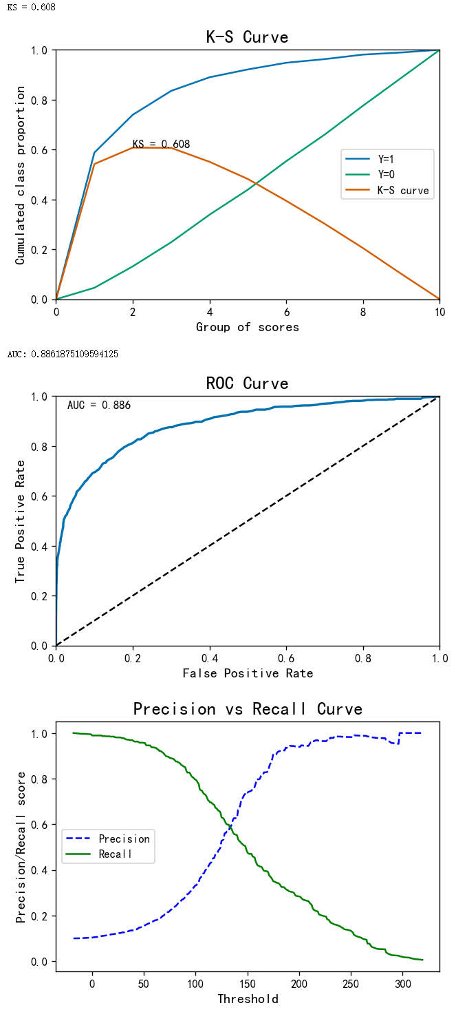
可视化模型评估结果(K-S曲线、ROC曲线、精确度召回率曲线)
# Validation
evaluation = me.BinaryTargets(y_val, result_val['TotalScore'])
evaluation.plot_all()
模型解释
解释单个样本的模型评分
# Features that contribute 80%+ of total score
imp_fs = mise.important_features(result_val
                 ,feature_names=list(sc_table.feature.unique())
                 ,col_totalscore='TotalScore'
                 ,threshold_method=0.8, bins=None)
result_val['important_features'] = imp_fs

# Features with top n highest score
imp_fs = mise.important_features(result_val
                 ,feature_names=list(sc_table.feature.unique())
                 ,col_totalscore='TotalScore'
                 ,threshold_method=2, bins=None)
result_val['top2_features'] = imp_fs

# Define the prediction threshold based on classification performance
result_val['y_pred'] = result_val['TotalScore'].map(lambda x: 1 if x>152 else 0)
result_val
| Latitude | HouseAge | Population | Longitude | AveRooms | TotalScore | important_features | top2_features | y_pred | |
|---|---|---|---|---|---|---|---|---|---|
| 0 | 38.0 | 15.0 | 30.0 | 35.0 | 11.0 | 129.0 | {‘Latitude': 38.0, ‘Longitude': 35.0, ‘Populat… | {‘Latitude': 38.0, ‘Longitude': 35.0} | 0 |
| 1 | 9.0 | 15.0 | 30.0 | 35.0 | 11.0 | 100.0 | {‘Longitude': 35.0, ‘Population': 30.0} | {‘Longitude': 35.0, ‘Population': 30.0} | 0 |
| 2 | 9.0 | 15.0 | 34.0 | 52.0 | 11.0 | 121.0 | {‘Longitude': 52.0, ‘Population': 34.0} | {‘Longitude': 52.0, ‘Population': 34.0} | 0 |
| 3 | 9.0 | 66.0 | 36.0 | 52.0 | 11.0 | 174.0 | {‘HouseAge': 66.0, ‘Longitude': 52.0} | {‘HouseAge': 66.0, ‘Longitude': 52.0} | 1 |
| 4 | 34.0 | 15.0 | 37.0 | 15.0 | 91.0 | 192.0 | {‘AveRooms': 91.0, ‘Population': 37.0} | {‘AveRooms': 91.0, ‘Population': 37.0} | 1 |
| … | … | … | … | … | … | … | … | … | … |
| 8251 | 34.0 | 33.0 | 37.0 | 15.0 | 37.0 | 156.0 | {‘Population': 37.0, ‘AveRooms': 37.0, ‘Latitu… | {‘Population': 37.0, ‘AveRooms': 37.0} | 1 |
| 8252 | 9.0 | 40.0 | 30.0 | 52.0 | 11.0 | 142.0 | {‘Longitude': 52.0, ‘HouseAge': 40.0} | {‘Longitude': 52.0, ‘HouseAge': 40.0} | 0 |
| 8253 | 34.0 | 15.0 | 24.0 | 15.0 | 37.0 | 125.0 | {‘AveRooms': 37.0, ‘Latitude': 34.0, ‘Populati… | {‘AveRooms': 37.0, ‘Latitude': 34.0} | 0 |
| 8254 | 9.0 | 15.0 | 36.0 | 35.0 | 11.0 | 106.0 | {‘Population': 36.0, ‘Longitude': 35.0} | {‘Population': 36.0, ‘Longitude': 35.0} | 0 |
| 8255 | 34.0 | 40.0 | 30.0 | 15.0 | 11.0 | 130.0 | {‘HouseAge': 40.0, ‘Latitude': 34.0} | {‘HouseAge': 40.0, ‘Latitude': 34.0} | 0 |
基于上述结果,我们可以对单个样本的模型结果进行解释。例如,第四行中(index=3),该样本总分为174,此结果的主要原因为房龄(HouseAge)和位置(Longitude)。这两个特征贡献了模型总分的80%以上,且为分数最高的两个特征。